Algorithms and Complexity

Fred Agbo

2025-09-03

Announcements

• Welcome back!
• Report any issues with practicing PS0 assignment
• Assignment for the week is posted and will be due next week Monday
  • Read over the full syllabus carefully

Algorithms

Learning Objectives

• Determine the rate of growth of the work of an algorithm in terms of its problem size
• Use big-O notation to describe the running time and memory usage of an algorithm
• Recognize the common rates of growth of work, or complexity classes:
  • constant, logarithmic, linear, quadratic, and exponential
• Describe searching algorithms and how they work
• Describe sorting algorithms and how they work

Measuring the Efficiency of Algorithms

• When choosing algorithms,
  • You often have to settle for a space/time trade-off
• An algorithm can be designed to gain faster run times
  • At the cost of using extra space (memory) or the other way around
• Space/time trade-off is more relevant for miniature devices

Measuring the Efficiency of Algorithms

• HOW?
  • Use the computer’s clock to obtain an actual run time:
    • Process is called benchmarking or profiling
  • Starts by determining the time for several different data sets of the same size and then calculates the average time
  • Next, similar data are gathered for larger and larger data sets:
    • After several tests, enough data are available to predict how the algorithm will behave for a data set of any size
• See code on the following slide

Measuring the Efficiency of Algorithms

# Prints the running times for problem sizes that double, using a single loop.

import time

problemSize = 10000000
print("%12s%16s" % ("Problem Size", "Seconds"))
for count in range(5):
    start = time.time()
    # The start of the algorithm
    work = 1
    for x in range(problemSize):
        work += 1
        work -= 1
    # The end of the algorithm
    elapsed = time.time() - start
    print("%12d%16.3f" % (problemSize, elapsed))
    problemSize *= 2

• Outputs:

Problem Size	Seconds
10,000,000	0.680
20,000,000	1.361
40,000,000	2.709
80,000,000	5.330
160,000,000	10.665

Built-In Python Collection: Lists

• Can you modify the program a little bit
• Ensure the extended assignments have been moved into a nested loop:
  • Loop iterates through the size of the problem within another loop that also iterates through the size of the problem
  • Line 11 to 13 now look like below:
• Update the problemSize = 1000 before running the new program

for j in range(problemSize):
    for k in range(problemSize):
        work += 1
        work -= 1

• What did you noticed?

Accurate Prediction but Problematic?

• This method permits accurate predictions of running times of many algorithms with only two problems:
  • Different hardware platforms have different processing speeds, so the running times of an algorithm differ from machine to machine
  • It is impractical to determine the running time for some algorithms with very large data sets

Complexity Analysis

Complexity Analysis

• This section focuses on developing a method of determining the efficiency of algorithms that allows you to rate them
  • Independently of platform-dependent timings or impractical instruction counts
• This method is called complexity analysis:
  • Entails reading the algorithm and using pencil and paper to work out some simple algebra

Orders of Complexity

A graph of the amounts of work done in the tester programs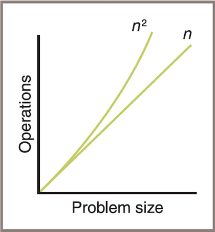

Orders of Complexity

• Performances of these algorithms differ by an order of complexity:
  • First algorithm is linear – work grows in direct proportion to the size of the problem
  • Second algorithm is quadratic – work grows as a function of the square of the problem size
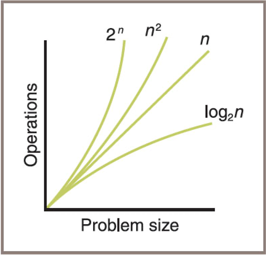
  • Constant – requires the same number of operations for any problem size
  • Logarithmic – amount of work is proportional to the log2 of the problem size
  • Polynomial time – grows at a rate of n^k, k = constant or > 1
  • Exponential – example rate of growth of this order is 2ⁿ

Orders of Complexity

A graph of some sample orders of complexity

Orders of Complexity

n	Logarithmic (log₂n)	Linear (n)	Quadratic (n²)	Exponential (2ⁿ)
100	7	100	10,000	Off the chart
1,000	10	1,000	1,000,000	Off the chart
1,000,000	20	1,000,000	1,000,000,000,000	Really off the chart

Big-O-Notation

• One notation used to express the efficiency or computational complexity of an algorithm is called big-O notation:
  • “O” stands for “on the order of,” a reference to the order of complexity of the work of the algorithm
• Big-O notation formalizes our discussion of orders of complexity
• It describes the upper bound of an algorithm’s running time or space requirements as the input size grows.
• It provides a way to classify algorithms according to their worst-case performance, relative to the input size (n), ignoring constant factors.

Big-O-Notation

• Common Big-O complexities include:
  • O(1): Constant time – does not depend on input size.
  • O(log n): Logarithmic time – grows slowly as input increases.
  • O(n): Linear time – grows directly with input size.
  • O(n²): Quadratic time – grows with the square of input size.
  • O(2ⁿ): Exponential time – grows very rapidly with input size.
• Big-O helps compare algorithms and choose the most efficient one for large data sets.
• It is used in both time and space analysis to predict scalability.

Searching and Sorting Algorithms

• This section covers several algorithms that can be used for searching and sorting lists/arrays
• You will
  • Learn the design of an algorithm
  • See its implementation as a Python function
  • See an analysis of the algorithm’s computational complexity

Search Algorithms

indexOfMin Algorithm:

def indexOfMin(lyst):
    """Returns the index of the minimum item."""
    minIndex = 0
    currentIndex = 1
    while currentIndex < len(lyst):
        if lyst[currentIndex] < lyst[minIndex]:
            minIndex = currentIndex
        currentIndex += 1
   return minIndex

Sequential search algorithm:

def sequentialSearch(target, lyst):
    """Returns the position of the target item if found,
    or -1 otherwise."""
    position = 0
    while position < len(lyst):
        if target == lyst[position]:
            return position
        position += 1
   return -1

IS THERE A BEST CASE?

Best-Case, Worst-Case, and Average-Case Performance

• The performance of some algorithms depends on the placement of the data processed:
  • The sequential search algorithm does less work to find a target at the beginning of a list than at the end of the list
• Analysis of a sequential search considers three cases:
  • In the worst case, the target item is at the end of the list or not in the list at all:
    • Algorithm must visit every item and perform n iterations for a list of size n. Thus, the worst-case complexity of a sequential search is O(n)

Best-Case, Worst-Case, and Average-Case Performance

• In the best case, the algorithm finds the target at the first position, after making one iteration, for an O(1) complexity
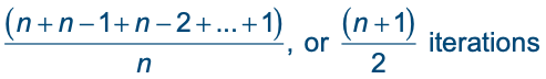
  • To determine the average case, add the number of iterations required to find the target at each possible position and divide the sum by n:
  • Thus, the algorithm performs

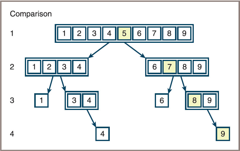
Binary Search of a Sorted List

Binary search algorithm:

def binarySearch(target, sortedLyst):
    left = 0
    right = len(sortedLyst) - 1
    while left <= right:
        midpoint = (left + right) // 2
        if target == sortedLyst[midpoint]:
            return midpoint
        elif target < sortedLyst[midpoint]:
            right = midpoint - 1
        else:
            left = midpoint + 1
   return -1

Sorting Lists or Arrays

• What:
  • Functions that put a list/array of elements into order
  • Numerical, lexical, or more complex relationships
• Why:
  • A fundamental data processing operation
  • Usually done at very large scale, so efficiency matters
  • A precursor to other types of calculations
  • Aggregations, uniqification, search

Simple approach: Bubble sort

• Compare each element (except the last one)with its neighbor to the right
  • If they are out of order, swap them
  • This puts the largest element at the very end
  • The last element is now in the correct and final place
• Compare each element (except the last two) with its neighbor to the right
  • If they are out of order, swap them
  • This puts the second largest element next to last
  • The last two elements are now in their correct and final places
• Compare each element (except the last three) with its neighbor to the right
• Continue as above until you have no unsorted elements on the left

Example of Bubble sort

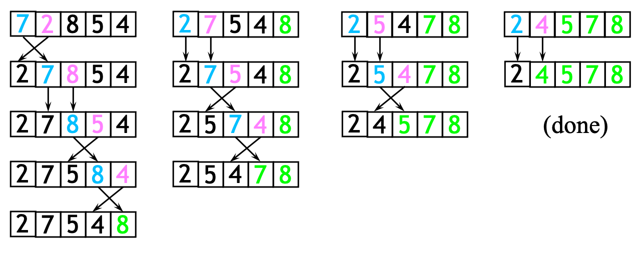
Bubble sort algorithm:

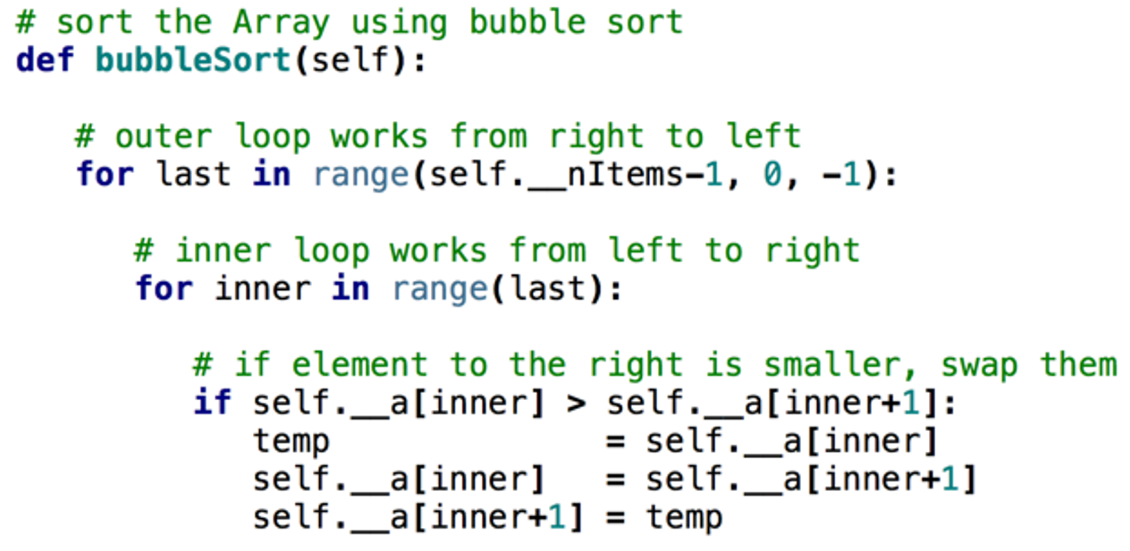
Bubble sort algorithm analysis

• Let n = nItems = number of items stored in the Array
• The 1st time through the outer loop, n-1 comparisons are done
• The 2nd time through the outer loop, n-2 comparisons are done
• The 3rd time through the outer loop, n-3 comparisons are done
• The final time through the outer loop 1 comparison is done
• Sum of 1 + 2 + 3 + … (n-3) + (n-2) + (n-1) ?
  • (n-1) * n / 2
• Result is O(n2) comparisons

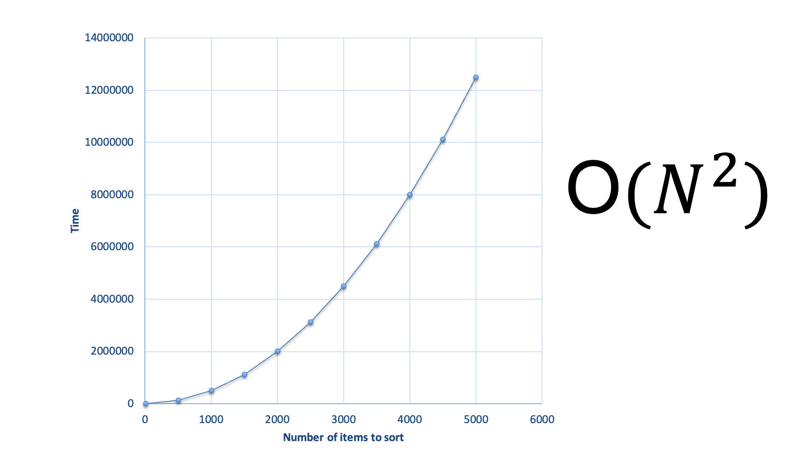
Performance of Bubble Sort Algorithm

Selection Sort Algorithm

• Given a list of length n,
  • Search elements 0 through n-1 and select the smallest
    • Swap it with the element in location 0
  • Search elements 1 through n-1 and select the smallest
    • Swap it with the element in location 1
  • Search elements 2 through n-1 and select the smallest
    • Swap it with the element in location 2
  • Search elements 3 through n-1 and select the smallest
    • Swap it with the element in location 3
  • Continue in this fashion until there’s nothing left to search

Selection Sort example and analysis

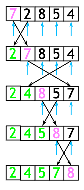
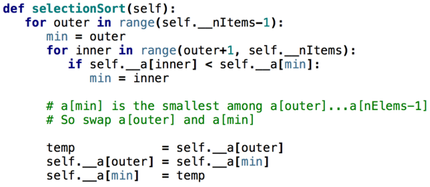
• The selection sort might swap an array element with itself–this is harmless, and not worth checking for Analysis:
  • 1st time through the outer loop, we do n-1 comparisons
  • 2nd time through the outer loop we do (n-2) comparisons
  • And so on… resulting in roughly
    • (1 + 2 + 3 + 4 + … + n-1) comparisons
  • You should recognize this as O(n²)

Selection sort algorithm:

Insertion Sort Algorithm

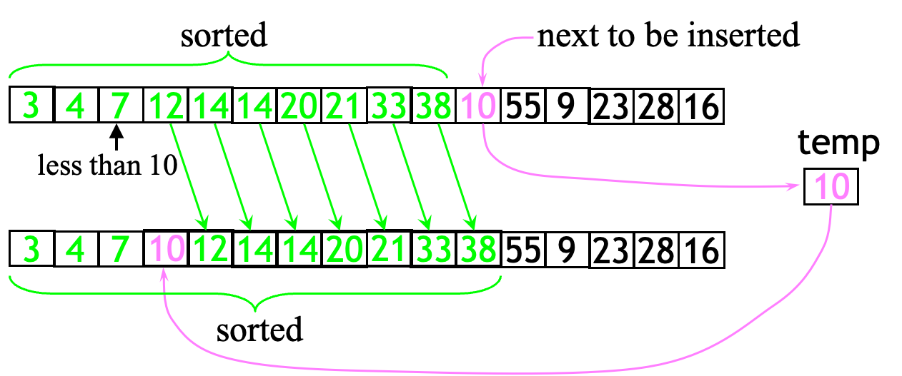
• For each element in the list (starting with the 2nd)
  • Find the first location to the left of the element that is less than or equal
  • Move everything to the right of that element one space and insert the element

One step of Insertion sort algorithm:

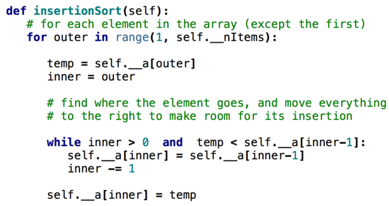
Insertion Sort Algorithm

Big O analysis of Insertion sort

• The 1st time through the outer loop we do one comparison.
• The 2nd time through the outer loop we do one or two comparisons
• The 3rd time through the outer loop we do one, or two, or three comparisons
• The Nth time through the outer loop we do one, two, … or N comparisons, but on average about N/2 comparisons.
• So, the total amount of work (numbers of comparisons and moves) is roughly:
  • (1 + 2 + 3 + 4 + … + N) / 2, or
  • N * (N + 1) / 4
• Discarding constants, we find that insertion sort is O(n²)

Big O analysis of Insertion sort

• What would the Big-O of insertion sort be, if we were to use binary search to find the insertion point?
  • Using binary search reduces the search for the insertion point to O(log n) per insertion.
  • However, shifting elements to make room for the new item still takes O(n) time per insertion.
  • Thus, the overall time complexity remains O(n²).

A Few Things to Note!

• Bubble sort, selection sort, and insertion sort are all O(n²)
• As we will see later, we can do much better than this with somewhat more complicated sorting algorithms
• Within O(n²),
  • Bubble sort is very slow, and should probably never be used for anything
  • Selection sort is intermediate in speed
  • Insertion sort is usually the fastest of the three–in fact, for small arrays (say, 10 or 15 elements), insertion sort is faster than more complicated sorting algorithms
• Selection sort and insertion sort are “good enough” for small arrays

Next week!

• Reading for next week:
  • Data Structures & Algorithms in Python (DS&A) - John et al.:
    • Chapter 6